

Table of Contents
1. HEGP challenge
2020-11-01 The authors announce the HEGP (heegeepee; hiːdʒiːpiː) Challenge, with a $1,000 (one thousand dollar) prize for the individual or group who can crack HEGP encrypted data.
See this page for a general introduction and relevance of HEGP
2. Details
The authors offer a reward of $1000 (one thousand US dollar) for cracking the HEGP homomorphic encryption method for genotypes and phenotypes as described in this open access paper.
The challenge consists of decryption of two genotype data sets.
In both data sets, plain text genotypes are represented numerically as matrices of allele dosages, with rows representing individuals and columns representing SNP sites or genotype markers (see below toy example). Each plain text genotype dosage takes the integer values 0,1,2. After encryption these dosages are transformed into floating point cyphertexts that are approximately normally distributed. The challenge is to recover the unencrypted original values from the cyphertext.
In HEGP, the ciphertext has been generated by matrix multiplication of
the plaintext genotype matrix by a random orthogonal matrix (the key
generated using Linux /dev/random and rustiefel) which is unknown to
you. The task therefore is to find the inverse of this matrix, which
because it is orthogonal, will be the transpose of original key.
For the first challenge1 we encrypted a data set consisting of 500 individuals by 12,359 SNP genotypes which exists in the public domain. We consider this data cracked if 50 individuals (10%) are identified correctly. Note that this data might be from human, mouse, rat, nematode or plants. Note also that these genotypes are a subset of a public dataset, and that any missing genotypes in the public data have been imputed before encryption.
The second challenge2 may be harder. We encrypted a mammalian data set that is not in the public domain (yet), consisting of 1,586 individuals and 12,561 SNPs. We consider the code cracked if you can compute the plaintext genotypes of this matrix correctly with mean error of under 10%.
The ciphertext files for challenge1 and challenge2 can be downloaded from https://files.genenetwork.org/HEGP-challenge/
The MD5 checksums of the ciphertext files are found in md5sum.txt. The full list, also for the original (secret for now) plaintext and keys is
5605626a9403ebdf96041d2dd766a516  challenge1.ciphertext.RData
148ce09c6dfc878af09874c090a7bd64  challenge1.ciphertext.txt
abbc5ce33025e723805cb14a332f6c9d  challenge1.maf.txt
29f348fd4d9fbd453f658def53dbb87a  challenge1.key.RData
b03e91f69d8124658e30562e1fa3b64c  challenge1.key.txt
dcf724ff4798f4ec6674d029f220385f  challenge1.plaintext.RData
e26367b991dfcedeaee139ffcc9a38a7  challenge1.plaintext.txt
d2db18e96a3a8173b12383aa8d606583  challenge1.sample.ids.txt

6d5d10279424a7c952ed8f9b0b086e84  challenge2.ciphertext.RData
c3706ecf12275859e3a040b23af1c9f9  challenge2.ciphertext.txt
15fa26a4d03e18f05643e917b8480216  challenge2.maf.txt
9615196bf89fb19105686a018e4c40c0  challenge2.key.RData
ecf00d15e233b6dda73e40ebdc3358d2  challenge2.key.txt
a007e8f5f085798a88180386ffbfa58f  challenge2.plaintext.RData
2b1870215dd67cfe1b19c423979ab3c7  challenge2.plaintext.txt
With this challenge we want to address the concern that individuals might be identified based on information in the public domain and/or by finding patterns in the encrypted data.
We will release the plaintext file and the key file when the challenge is cracked or after six months (which is May 1st 2021). In case the prize is unclaimed we'll create a new dataset for a fresh challenge.
The ciphertext Datasets are provided as RData objects which can be manipulated using the hegp R package. Briefly, a dataset D is a list, comprising of minimally a phenotype vector D$y, and a genotype dosage matrix D$geno (rows are individuals, columns are SNPs). There are additional components that are useful for GWAS but not relevant for the decryption challenge. Full details are in the documentation of the R package. The challenge datasets have fake phenotype data that can be ignored.
To unpack the RData original datasets and write the genotypes and allele frequencies to tab-delimited text files from R, convert with
library(readr)
load("challenge2.ciphertext.RData")
write.csv( De$geno, "challenge1.ciphertext.txt", quote=F)
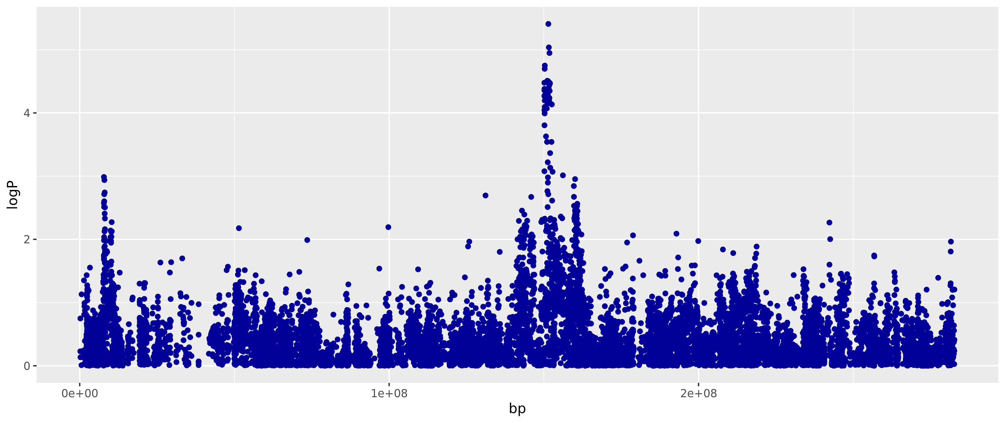
To run a GWA use the mixed-model-gwas and hegp-R packages you can run in R
library(hegp)
load("challenge2.ciphertext.RData")
ge.mm=basic.mm.gwas(De,mc.cores=1)
  Built kinship dim 1586 1586
  estimated heritability 4.355436e-05
ls(ge.mm)
  [1] "bp"   "chr"  "logP"
ge.mm$logP[0:6]
  [1] 0.22838514 0.74881022 0.13431556 0.00929719 1.13027222 0.13211178
and draw a plot with
library(ggplot2)
ggplot(ge.mm) + geom_point(aes(bp, logP), colour="#000099")
To validate we ran the encrypted version (De) and then plaintext version (D) to compare outcomes with
library(hegp)
load("challenge2.ciphertext.RData")
load("challenge2.plaintext.RData")
ls()
  [1] "D"  "De"
ls(D)
  [1] "cov"  "geno" "maf"  "map"  "y"
ls(De)
  [1] "cov"  "geno" "map"  "y"
g=basic.gwas(D)
ge=basic.gwas(De)
mean(abs(g$logP-ge$logP))
  0.02951522
ge.mm=basic.mm.gwas(De,mc.cores=1)
  Built kinship dim 1586 1586
  estimated heritability 4.355436e-05
g.mm=basic.mm.gwas(D,mc.cores=1)
  Built kinship dim 1586 1586
  estimated heritability 4.356434e-05
mean(abs(g.mm$logP-ge.mm$logP))
   [1] 0.02943622
Documentation for the R encryption and GWA functions can be found here.
3. Reference code
The reference code for HEGP is published under GPLv3 licensed R code and Julia code. An example of running a GWA as presented in the paper can be found here. The algorithm with a description of brute force attack is described in the results section.
4. Submissions
Submissions should be posted in a permanent public git account (GitHub, gitlab or similar) and reward will be given in USD. The solution should be reproducible and announced on the website issue tracker. In case you don't want to use the issue tracker it is also possible to E-mail the authors to indicate where the solution is hosted. One such E-mail address is pjotr.public542 at thebird dot nl.
Important note: only real solutions will be considered that can reliably crack the key of any such dataset. If the original key somehow gets ripped from one of our laptops, for example, it does not count. Security stands or falls with how data is handled and how a key is generated. Even so, this challenge is about algorithmically cracking the code for the general case.
5. Feedback
Feedback on the challenge, this website etc., can be posted to the issue tracker.
6. General introduction
The homomorphic encryption method consists of an orthogonal transformation by multiplication by the orthogonal matrix P with a matrix containing the data y and G.
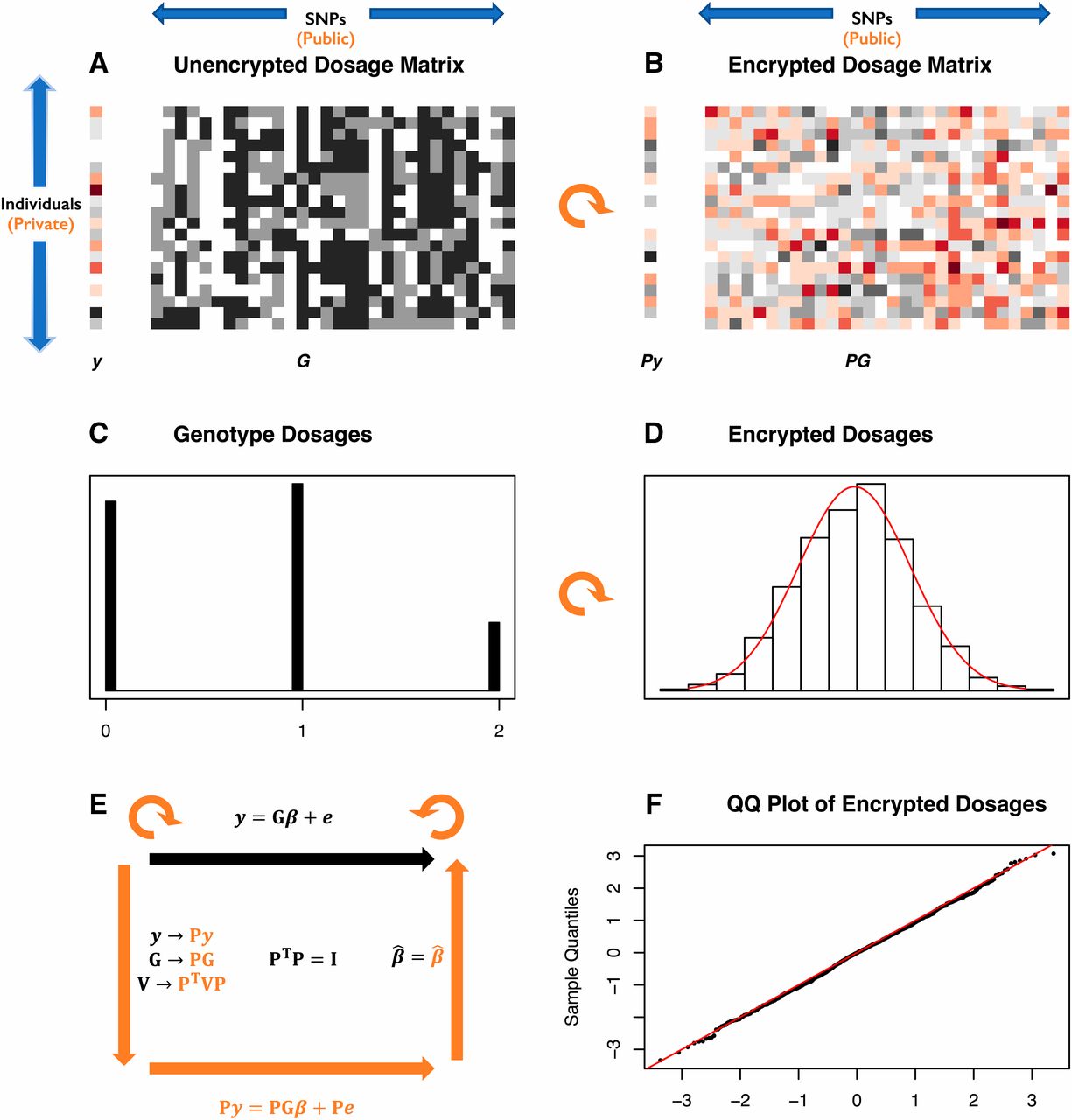
From the original paper: privacy in relation to quantitative genetic analysis. (A) A numeric phenotype vector y (left) and genotype dosage matrix G (right) are represented as colours and shades of gray. Each row of the matrix represents one individual and each column one SNP. Genotypes are encoded as imputed dosages clustered at the values Embedded Image giving the numbers of alternate alleles. (B) The same data after multiplication by an orthogonal matrix P (a rotation represented by the curved orange arrow). The genotype dosages are now represented by a continuum of real numbers. (C) The distribution of dosages for a particular SNP (column of G), clustered around 0,1,2. (D) The distribution of the same dosages after orthogonal transformation by multiplication by the orthogonal matrix P (black histogram) with the normal distribution with same mean and variance superimposed in red. (F) The normal QQ plot for the data in D, showing the transformed dosages are very close to a normal distribution. (E) A cartoon of the HEGP scheme. The top black arrow and equation show the linear mixed model relating the phenotype y to genotype G with regression coefficients β representing the allelic effects. The variance matrix for the residuals is V. After multiplication by orthogonal matrix P, plaintext data y, G and the mixed linear model are transformed as shown in orange. The likelihood and regression estimates β are preserved. HEGP, homomorphic encryption for genotypes and phenotypes; QQ, quantile–quantile.
7. Toy Example
The task is best described with an small example, a SNP dosage matrix G with 10 subjects (rows) and 8 SNPs (columns):
sub1     0    1    2    1    1    1    1    2
sub2     0    1    2    1    2    2    2    2
sub3     1    1    2    1    2    2    2    1
sub4     2    1    2    2    1    2    1    1
sub5     2    2    2    0    1    1    2    1
sub6     2    2    2    1    1    2    2    2
sub7     1    2    1    1    1    1    2    2
sub8     0    1    2    1    2    1    2    2
sub9     1    1    2    2    1    1    1    2
sub10    1    2    2    1    2    2    2    1
The first step standardises each column to have mean 0 and variance 1. This does not encrypt the data but it makes the encryption easier to process. The resulting plaintext dosage matrix H is
sub1  -1.224745e+00 -0.7745967  0.3162278 -0.1761661 -0.7745967 -0.9486833 -1.449138  0.7745967
sub2  -1.224745e+00 -0.7745967  0.3162278 -0.1761661  1.1618950  0.9486833  0.621059  0.7745967
sub3  -5.749536e-10 -0.7745967  0.3162278 -0.1761661  1.1618950  0.9486833  0.621059 -1.1618950
sub4   1.224745e+00 -0.7745967  0.3162278  1.5854946 -0.7745967  0.9486833 -1.449138 -1.1618950
sub5   1.224745e+00  1.1618950  0.3162278 -1.9378267 -0.7745967 -0.9486833  0.621059 -1.1618950
sub6   1.224745e+00  1.1618950  0.3162278 -0.1761661 -0.7745967  0.9486833  0.621059  0.7745967
sub7  -1.761818e-09  1.1618950 -2.8460499 -0.1761661 -0.7745967 -0.9486833  0.621059  0.7745967
sub8  -1.224745e+00 -0.7745967  0.3162278 -0.1761661  1.1618950 -0.9486833  0.621059  0.7745967
sub9   5.584054e-10 -0.7745967  0.3162278  1.5854946 -0.7745967 -0.9486833 -1.449138  0.7745967
sub10 -7.763129e-10  1.1618950  0.3162278 -0.1761661  1.1618950  0.9486833  0.621059 -1.1618950
Next, we sample a random orthogonal 10x10 matrix P (the key)
 [1,] -0.02512827 -0.4797328  0.07364427  0.29302653 -0.52531836 -0.06077012 -0.035656119 -0.21264789 -0.03656364  0.59199429
 [2,]  0.49690414 -0.2130092 -0.18437213 -0.08094409 -0.33989098  0.11458794  0.382316649  0.51918534 -0.29625914 -0.18714471
 [3,]  0.23650365  0.2027581  0.09184543  0.01711933  0.45947279 -0.11898452  0.549979207  0.04901441  0.03087585  0.60259531
 [4,] -0.12668661  0.2640016 -0.24657807 -0.31047136 -0.08100156  0.01898761 -0.009330209 -0.34743514 -0.77909552  0.14950124
 [5,]  0.55558644 -0.1256327 -0.11075554 -0.35350803  0.12981113  0.51028646 -0.332763562 -0.28269321  0.20446208  0.16914618
 [6,] -0.20079972 -0.1310010  0.33769938 -0.45070382  0.09236098 -0.05672098 -0.390626201  0.58184807 -0.14355153  0.31914343
 [7,]  0.30606137  0.1956211  0.67114299 -0.30536330 -0.32325985 -0.31468499  0.106176504 -0.27993855  0.04238805 -0.17152201
 [8,] -0.31057809 -0.5813563  0.28456863 -0.21173902  0.26275032  0.30931163  0.411201611 -0.21696952 -0.12053771 -0.21059453
 [9,]  0.07808339 -0.3843085 -0.42321573 -0.37251969  0.13692025 -0.68291915 -0.007551188 -0.12694060  0.15450958 -0.05619238
[10,] -0.36775701  0.2383173 -0.23348592 -0.45381168 -0.41614295  0.20969099  0.325976664  0.04578156  0.44759290  0.14716487
Then we encrypt the dosages F = PH to make the ciphertext
sub1   0.5198393  0.26551339 -0.01916052  1.4507213  0.2713387  1.18915219 -0.7379842 -1.16229696
sub2  -1.3586430 -0.22207809 -1.14214913 -0.1029684 -0.2902612 -1.24575229 -0.1165288  1.69811232
sub3  -0.1600357  1.24824503 -1.06841109 -1.0985638  0.1892755 -0.50328813  0.7284091 -0.62463676
sub4  -0.1988559  1.28854213 -0.43475181 -1.5181190  0.7876347  1.15643550  1.6061022 -0.19111906
sub5   0.1706426  0.64079385  1.16737846 -0.5553653 -0.9595529 -0.17537980 -0.6155911  0.60202029
sub6  -0.8145915 -0.03660399  1.22187582 -1.2021241  2.1778375  0.07512188  1.6196177 -0.61084795
sub7  -1.4268916 -1.30507703 -0.35896396  0.1191278  0.8610707  0.21228333 -0.1347692  0.19297276
sub8   1.7994281  1.79366813 -1.42174710 -0.9805980 -1.1053001 -0.41331874  1.0923847 -0.53943417
sub9  -0.5944334  0.12376342 -0.50869100 -0.3285796 -0.6138749 -2.04363166 -0.7562708  0.08008153
sub10 -0.7061947  0.56034104 -1.04875037  0.7321312  0.4268941 -0.12102879  0.7390060  1.80792099
This form of encryption is homomorphic with respect to many quantitative genetics analyses, particularly the mixed model GWAS.
To decrypt the ciphertext it is necessary to multiply it by the inverse of the key P, which is equal to the transpose of P because it is orthogonal.
The challenge is, in the absence of knowing either P or H, to find an orthogonal matrix Q such that QF "looks like" a genotype dosage matrix. That is, the distribution of the plaintext for a given SNP will be trimodal (or bimodal is the rarer homozygote genotype is absent from the sample) with expected modes specified by the Hardy-Weinberg equilibrium distribution. We provide the allele frequencies of the plaintext, which will help in defining these expected modes (see the maf.txt files). It is reasonable to provide this information even though it might make the encryption less secure because users of the ciphertext would need this information for some genetic analyses.
We provide the toy dataset and its encryption key as R objects in the file "toy.hegp.RData" from Toy-HEGP so that you can reproduce these analyses. E.g.
# Load a table
toy = read.table("toy2.txt",header=F,row.names=1)

library(hegp)
load("toy.hegp.RData") # loads encryption key
plaintext.toy$geno = as.matrix(toy)
c = encrypt.D(plaintext.toy, key.toy)
d = encrypt.D(c, key.toy, invert=TRUE)
mean(abs(c$geno-d$geno))
[1] 2.524352e-09
8. References
- The original HEGP paper
- HEGP discussion on reddit crypto forum
- For more background see this page